Monthly Archives: December 2016

Open Boundary

Assume there are 3 lines separating 3 areas:
line1: y=x , (x <= 10)
line2: y=20-x,  (x>=10)
line3: x=10, y>=10

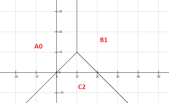
For each area, there are some data:
A:
[-3, -2, 0]
[-3, 1, 0]
[0, 40, 0]
[8, 90, 0]
[8, 10, 0]
[3, 40, 0]

B:
[11, 11, 1]
[15, 6, 1]
[13, 10, 1]
[13, 19, 1]
[23, -1, 1]
[25, -2, 1]

C:
[-2, -3, 2]
[3, 2, 2]
[10, 9, 2]
[15, 10, 2 ]
[20, -1, 2]
[25, -10, 2]

Run below code, we expect that [10, 5] will output value 2. Because point (10, 5) belongs to area B, which has value 2.

import numpy as np
import matplotlib.pyplot as plt
from sklearn import linear_model, datasets

X = np.array([
    [-3, -2],
    [-3, 1],
    [0, 4],
    [8, 9],
    [8, 10],
    [3, 4],
    [11, 11],
    [15, 6],
    [13, 10],
    [13, 19],
    [23, -1],
    [25, -2],
    [-2, -3],
    [3, 2],
    [10, 9],
    [15, 10],
    [20, -1],
    [25, -10]
])

Y = np.array([0, 0, 0, 0, 0, 0, 1, 1, 1, 1, 1, 1, 2, 2, 2, 2, 2, 2])

logreg = linear_model.LogisticRegression(C=1e5)

# we create an instance of Neighbours Classifier and fit the data.
logreg.fit(X, Y)

print logreg.predict(np.array([[10, 5]]))

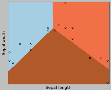
Run below code, it outputs the boundary and region:

h = .02  # step size in the mesh

# Plot the decision boundary. For that, we will assign a color to each
# point in the mesh [x_min, x_max]x[y_min, y_max].
x_min, x_max = X[:, 0].min() - .5, X[:, 0].max() + .5
y_min, y_max = X[:, 1].min() - .5, X[:, 1].max() + .5
xx, yy = np.meshgrid(np.arange(x_min, x_max, h), np.arange(y_min, y_max, h))
Z = logreg.predict(np.c_[xx.ravel(), yy.ravel()])

# Put the result into a color plot
Z = Z.reshape(xx.shape)
plt.figure(1, figsize=(4, 3))
plt.pcolormesh(xx, yy, Z, cmap=plt.cm.Paired)

# Plot also the training points
plt.scatter(X[:, 0], X[:, 1], c=Y, edgecolors='k', cmap=plt.cm.Paired)
plt.xlabel('Sepal length')
plt.ylabel('Sepal width')

plt.xlim(xx.min(), xx.max())
plt.ylim(yy.min(), yy.max())
plt.xticks(())
plt.yticks(())

plt.show()

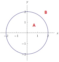
Enclosed Boundary

Suppose we have A, B parts
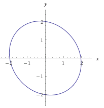
A: x^2 + y^2 <=2
B: x^2 + y^2 > 2

To solve this, we can use Polynomial Logistic Regression method. This is similar to Polynomial Linear Regression.

import numpy as np
import matplotlib.pyplot as plt
from sklearn.preprocessing import PolynomialFeatures
from sklearn import linear_model

# Area A: x^2 + y^2 <= 2
# Area B: x^2 + y^2 > 2
X = np.array([
    # training set for A
    [0, 0],
    [1, 0],
    [1.5, -0.2],
    [1, 1.5],
    [-1, -1.5],
    [-1.9, 0],
    [-0.5, -1],
    [0, 1.9],
    [0, -1.9],
    [-1.9, 0],
    [-1.5, 0.5],
    # training set for B
    [2, 2.5],
    [2, 3],
    [1, 5],
    [1, -5],
    [-3, 0],
    [-2, -0.1],
    [-2, 1],
    [0, -2.1],
    [0, 2.1],
    [-2.1, 0],
    [-0.6, -2]
])

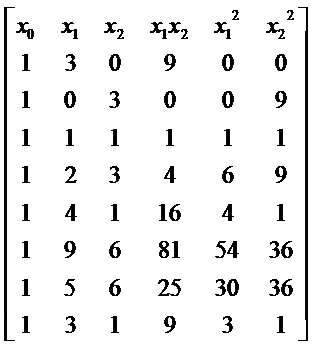
poly = PolynomialFeatures(degree=2)
X_trans = poly.fit_transform(X)

Y = np.array([0, 0, 0, 0, 0, 0, 0, 0, 0, 0, 0, 1, 1, 1, 1, 1, 1, 1, 1, 1, 1, 1])

logreg = linear_model.LogisticRegression(C=1e6)

# we create an instance of Neighbours Classifier and fit the data.
logreg.fit(X_trans, Y)

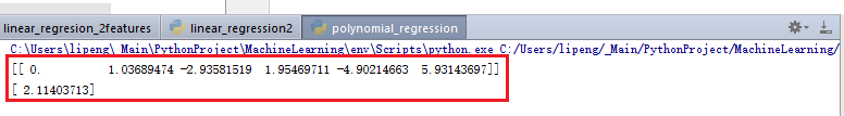
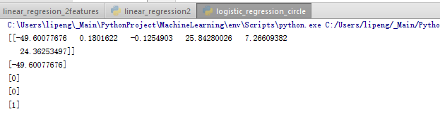
print logreg.coef_
print logreg.intercept_
print logreg.predict(np.array(poly.fit_transform([[0, 1.8]])))  # expect to return 0
print logreg.predict(np.array(poly.fit_transform([[0, -1.8]])))  # expect to return 0
print logreg.predict(np.array(poly.fit_transform([[0, -2.1]])))  # expect to return 1

And the result is:

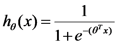
Accordingly, we can build the hypothesis:

Check my code on github: open boundary, enclosed boundary