Monthly Archives: November 2016

Virtualenv in PyCharm

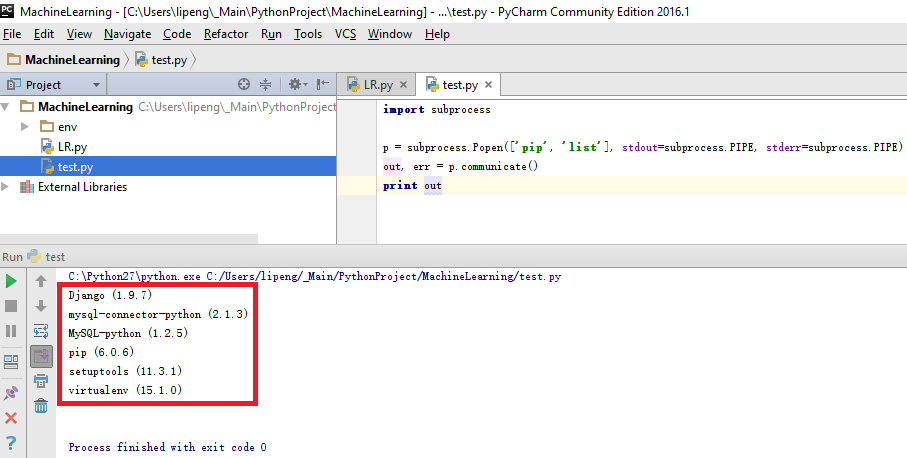
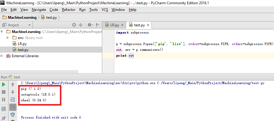
Run below code, we can check what package we have under current environment.

import subprocess

p = subprocess.Popen(['pip', 'list'], stdout=subprocess.PIPE, stderr=subprocess.PIPE)
out, err = p.communicate()
print out

env1

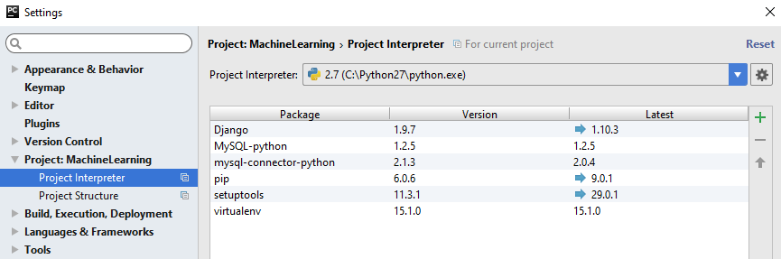
In PyCharm -> Project Interpreter -> list box Project Interpreter, here are all the python environments:
setting

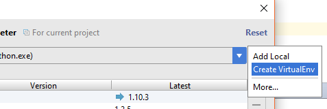
Under system button, select Create VirtualEnv
create_new_virtualenv

create_new_virtualenv2

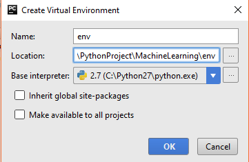
Now, we have new virtual environment.
create_new_virtualenv3

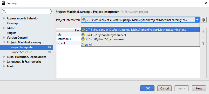
Let’s try the code again. We see the package list changed.
env2

Not ended yet….

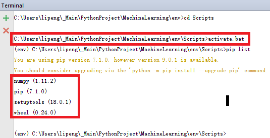
Let’s open terminal console in PyCharm and try virtualenv activate command. Unfortunately, it shows that it couldn’t find source command, which is different from Linux.
source_fail

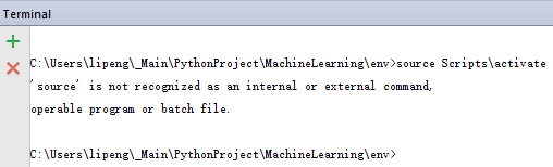
To activate virtualenv in Windows, we end up with running Scripts\activate.bat command in env folder.
source_fail2

Simple Linear Regression

I’m learning machine learning these days. Here let me write down the note for this.
Suppose we have m training points training_set in x-y coordination, and we want to find the best line fit for these points .
sample_points

Since it is the simplest line, we can define the line function, and call it hypothesis:
hypothesis.

A way to measure how well a line fit these points is least square mean. And we call it loss function:

loss_function

Now, the problem turns to find the pair which the loss function has the minimum value. As said by Andrew NG, the fortunate thing is that the loss function of linear regression are all bowl shape, which mean it always has a extreme value.
bowl_shape

One way to minimize the loss function is to use gradient descent algorithm. The basic idea is to let the point on the surface go through gradient direction, in this way, it will finally reach the extreme value. Partial derivative functions for loss function:
derivative

After we got the partial derivative function, we do below until loss function is less than boudary
iteration

When the loss function is getting close the extreme value, we can see the pair is moving to the extreme value from the gradient direction.

change_of_loss


Example of Gradient Descent

Let’s talk about this function:
gd1

It has shape like this:
gd5

Obviously, it has extreme point (0, 0, 0). Let’s use gradient descent to get the extreme point.

Calculate the partial derivative:
gd2

Then, let’s take any point in (x, y), and run like below. Lambda is a tiny value, which controls how fast P goes to the extreme value.
gd3
gd4

After we ran, we got the below iteration:

0 (x, y): 1.0, 5.0
1 (x, y): 0.803883864861816, 4.01941932430908
2 (x, y): 0.6077677297236319, 3.0388386486181598
3 (x, y): 0.41165159458544787, 2.0582579729272394
4 (x, y): 0.21553545944726385, 1.0776772972363193
5 (x, y): 0.019419324309079833, 0.09709662154539911
6 (x, y): -0.1766968108291043, -0.8834840541455209
7 (x, y): 0.01941932430907986, 0.09709662154539922
8 (x, y): -0.17669681082910432, -0.8834840541455209
9 (x, y): 0.01941932430907986, 0.09709662154539922
(x, y): -0.17669681082910432, -0.8834840541455209

It shows that it iterates close to the extreme value (0, 0), but it go around (0, 0) when it arrives.

My java code for this gradient descent algorithm:

public static void main (String[] args) throws java.lang.Exception{
    // your code goes here
    System.out.println(Math.pow((26 * 26 + 46 * 46), -0.5));
    double x = 1, y = 5, delta = 1;
    for (int i = 0; i < 10; i++) {
        System.out.println(i + " (x, y): " + x + ", " + y);
        double tmp = Math.pow((x * x + y * y), -0.5);
        double x2 = x - delta * x * tmp;
        double y2 = y - delta * y * tmp;
        x = x2;
        y = y2;
    }
    System.out.println("(x, y): " + x + ", " + y);
}

code on github